

An IELTS Writing Task 1 Line Graph can look intimidating at first. You see several lines, a long time span, and dozens of numbers, all with a limited amount of time to respond. The good news is that line graphs follow a small set of patterns. Once you recognize them, the task becomes a matter of choosing what to report and reporting it clearly.
This guide covers a simple structure, useful sentence patterns, practical tips, and the mistakes that cost candidates the most marks.
IELTS Line Graph Writing Template
A reliable answer has four parts, and each one has a specific job.
- Introduction: Restate the graph in one or two sentences. Change the wording from the question prompt, but keep the meaning exact. Mention what the graph shows, the units, and the time period.
- Overview: Give the big picture in two or three sentences. Mention the general direction of the lines, the highest and lowest points, and anything that stands out. Leave out precise figures here, because the overview is about the overall pattern.
- Body paragraph one: Cover the first group of lines or the first part of the period. Include starting points, end points, and the main peaks and dips. Group related lines together so the reader can follow your logic.
- Body paragraph two: Deal with the remaining data. Compare lines, note any crossovers, and mention anything that behaves differently from the rest.
Some sentence patterns you can adapt:
- Visitor numbers climbed from 2 million in 2010 to 5 million by 2020.
- Sales hit a peak of around 300 units in 2015 before dropping sharply.
- Production barely moved, whereas exports overtook imports in 2018.
- The rural figure, by contrast, declined gradually across the period.
- Both lines started at roughly the same level but split apart after 2012.
Treat these as starting points rather than scripts. Vary your subjects, move your time expressions around, and mix active and passive forms. Repeating one structure across the whole answer makes the writing sound mechanical, and examiners notice that.

Tips for Scoring 7+ Bands in IELTS Task 1 Line Graph
Read the Graph Before You Write
- Spend about two minutes finding the highest point, the lowest point, and any lines that cross. Check the vertical scale as well. A gap that looks small on the page can be large in real terms, and misreading the axis is an easy way to lose accuracy marks. Jot down three or four notes in your scratch space before you start writing.
Choose Only the Key Features
- You will not have room or time to report every data point. Pick three or four main trends and build your body paragraphs around them. A selective answer with accurate figures always beats a crowded one full of small errors. If a detail does not help the reader understand the overall picture, leave it out.
Decide Your Overview Early
- Even if you plan to write the overview last, know what it will say before you begin the body paragraphs. The overview tells you which details belong in the body and which can be dropped. It also keeps the whole answer coherent, because every paragraph then has a clear purpose.
Learn How Trend Verbs Behave
- Words like rise, climb, plateau, decline, and fluctuate are useful, but their grammar differs. “Rise” and “climb” do not take an object, so you write “rose from X to Y.” “Raise” does take one, as in “raised prices.” Spend a few minutes checking these patterns before the exam, because one wrong structure can appear many times in a single answer.
Use Approximation When Figures Are Not Exact
- Words like “around,” “roughly,” “just over,” and “nearly” show that you are describing the chart rather than inventing precision. Use them where they fit, but not in every sentence. Too many hedges make the report sound unsure of itself, while none at all can make an estimate look like an exact fact.
Keep Your Tense Steady
- Past simple usually works well for historical data. If the graph includes a forecast or runs up to the present, the tense may change, so read the time frame carefully before you begin. Random tense switching costs grammar marks, and it also confuses the reader about when events happened.
Compare Things That Can Be Compared
- “The number of students was higher than the number of teachers” works because both items are counts of people. Comparing the number of students with the amount of money makes no sense. Before you write a comparison, check that both sides measure the same kind of thing and use the same unit.
Paraphrase As You Go
- Swap “the number of” for “the figure for” or “the level of” when it suits the sentence. This shows range without changing the meaning, which is exactly what examiners want to see. Keep key terms like the unit of measurement accurate, though, because a wrong unit can damage your task achievement score.
Reserve Time for Checking
- Leave two or three minutes at the end to read your answer again. Look for missing articles, wrong plurals, and spelling slips. Confirm that every figure matches the graph and that your overview contains no specific numbers. These small checks often make the difference between two band scores.
IELTS Task 1 Line Graph Sample Questions with Answers
Sample Question 1
Answer:
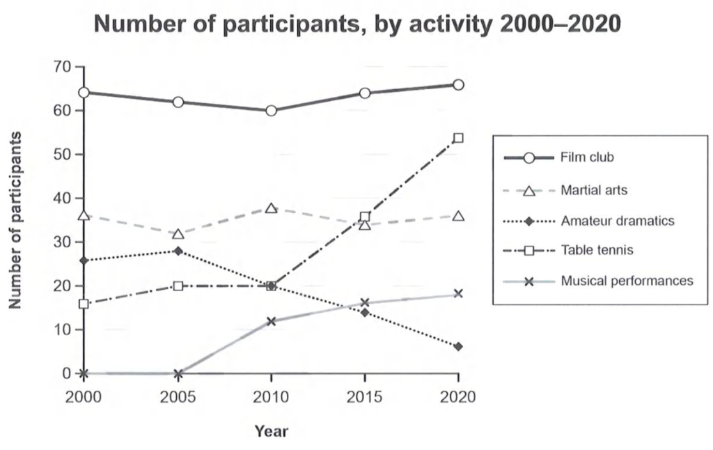
The line graph illustrates the number of participants in five different activities, namely film clubs, martial arts, amateur dramatics, table tennis and musical performances, between 2000 and 2020.
Overall, the film club remained the most popular activity throughout the period, while amateur dramatics experienced a considerable decline. Table tennis recorded the most significant growth, whereas musical performances attracted more participants towards the end of the period.
In 2000, the film club had approximately 64 participants, compared with 36 for martial arts and 26 for amateur dramatics. Film club membership fell gradually to 60 in 2010 before recovering to around 66 in 2020. Martial arts participation fluctuated, dropping to 32 in 2005, rising to 38 in 2010, and finishing at approximately 36. Meanwhile, amateur dramatics increased slightly from 26 to 28 between 2000 and 2005, before declining steadily to just 6 in 2020.
Table tennis participation rose from 16 in 2000 to 20 in 2005, remaining stable until 2010. It then increased sharply to 36 in 2015 and 54 in 2020. Musical performances had no participants in 2000 and 2005, but the figure climbed to 18 by the end of the period.
Sample Question 2
Answer:
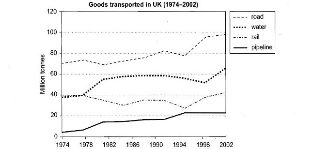
The line graph illustrates the amount of goods transported in the UK by four different modes of transport, namely road, water, rail and pipeline, between 1974 and 2002. The figures are measured in million tons.
Overall, road transport carried the largest quantity of goods throughout the period, while pipeline remained the least-used method for most of the years. Water transport experienced considerable growth, whereas rail transport fluctuated and showed a slight overall increase.
In 1974, approximately 70 million tons of goods were transported by road, compared with around 40 million tons by both rail and water. Road transport increased gradually, despite some fluctuations, reaching nearly 100 million tons in 2002. Water transport remained relatively stable until 1978, before rising to about 55 million tons in 1982. After fluctuating around 50–60 million tons, it climbed to approximately 65 million tons by the end.
Rail transport started at around 40 million tons and fluctuated throughout the period, falling to 30 million tons in the mid-1980s before recovering to roughly 40 million tons in 2002. In contrast, pipeline transport increased steadily from about 3 million tons in 1974 to 22 million tons in 1998, after which it remained unchanged until 2002.
Sample Question 3
Answer:
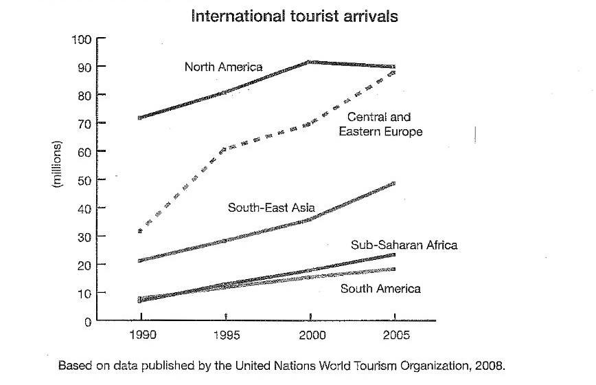
The line graph compares the number of international tourists visiting five regions, namely North America, Central and Eastern Europe, South-East Asia, Sub-Saharan Africa and South America, between 1990 and 2005. The figures are given in millions.
Overall, tourist arrivals increased in all five regions over the period. North America attracted the highest number of visitors, although Central and Eastern Europe experienced the fastest growth. South America had the lowest figures for most of the period.
In 1990, North America received approximately 72 million international tourists, making it the leading destination. This figure rose steadily to around 92 million in 2000 before slipping slightly to 90 million in 2005. Meanwhile, Central and Eastern Europe recorded a substantial increase from roughly 32 million visitors in 1990 to 60 million in 1995. Its figures continued to climb, reaching about 70 million in 2000 and nearly 90 million by 2005.
South-East Asia also experienced consistent growth, with tourist arrivals increasing from approximately 21 million in 1990 to 35 million in 2000, before reaching around 49 million in 2005. Similarly, Sub-Saharan Africa rose from about 8 million to 22 million over the period. South America followed a slower upward trend, with arrivals increasing from approximately 7 million in 1990 to 18 million in 2005.

Sample Question 4
Answer:
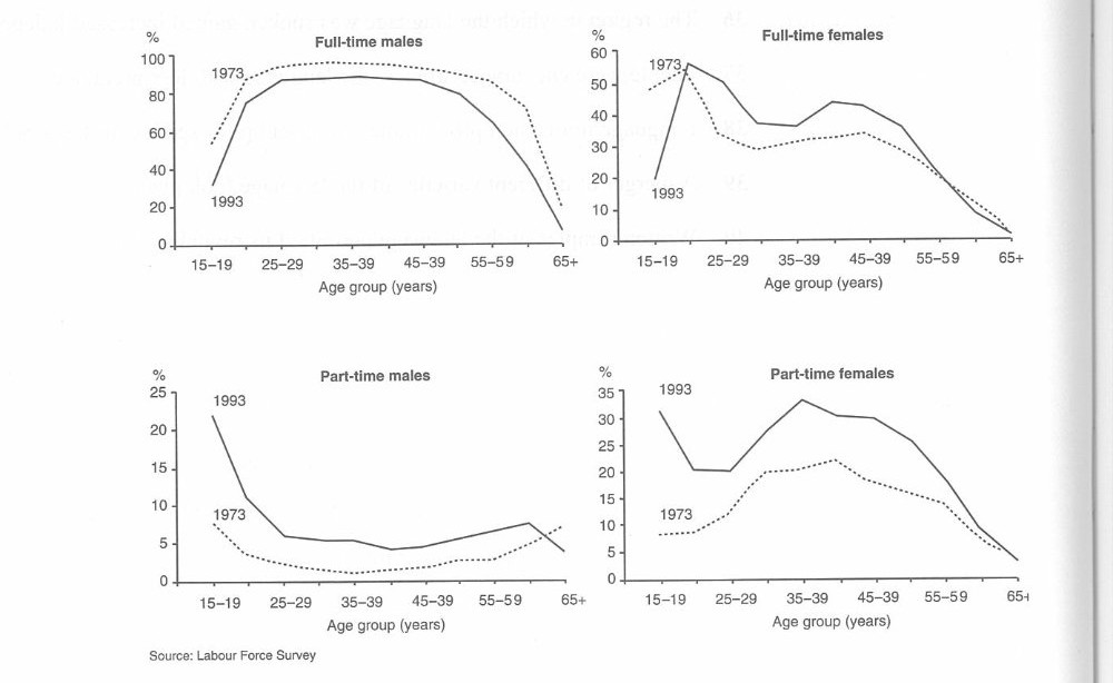
The four line graphs compare the percentages of male and female workers employed full-time and part-time across different age groups in 1973 and 1993.
Overall, men were more likely to work full-time, whereas women accounted for a higher proportion of part-time workers. Employment figures generally declined among older people, particularly those aged 65 and above.
For full-time males, the figure in 1973 increased sharply from around 60% among 15–19-year-olds to approximately 90% among those aged 25–29, remaining high until middle age before falling. In 1993, the rate started at about 30% and peaked at roughly 85%. Among full-time females, the 1973 figure began at around 50%, while the 1993 rate was only 20%. Both figures fluctuated before declining significantly in older age groups.
Part-time employment showed a different pattern. Among men, the 1993 rate started at approximately 22% and dropped considerably, while the 1973 figure remained much lower throughout most age groups. In contrast, part-time employment among women was higher in 1993, reaching a peak of about 33% among 35–39-year-olds, compared with around 20% in 1973. Both rates declined sharply among older workers.
Sample Question 5
Answer:
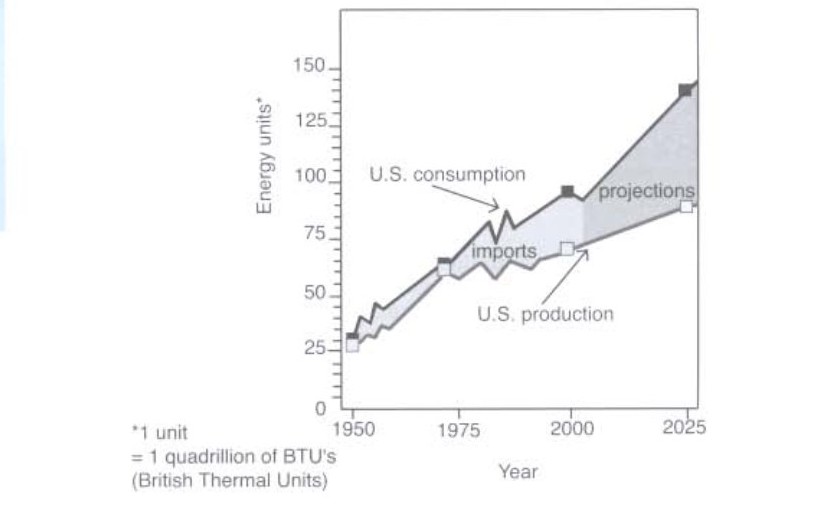
The line graph compares U.S. energy consumption and production from 1950 to 2025, measured in quadrillions of British Thermal Units (BTUs).
Overall, both consumption and production show an upward trend. However, consumption is projected to rise more rapidly than production, creating a significant gap by 2025, with consumption reaching the highest level.
In 1950, U.S. energy consumption stood at approximately 30 units, slightly higher than production at around 25 units. Both figures increased over the following decades, despite some fluctuations. By 1975, they had reached roughly 60 units. Consumption then fluctuated, peaking at around 85 units in the mid-1980s before falling slightly.
After this period, consumption continued to rise, reaching approximately 90 units around 2000. It is projected to increase sharply to about 140 units by 2025. In contrast, U.S. production remained lower, reaching around 65 units in 2000 and rising gradually to approximately 85 units in 2025. Consequently, the difference between energy consumption and production is expected to widen considerably over the projection period.
Sample Question 6
Answer:
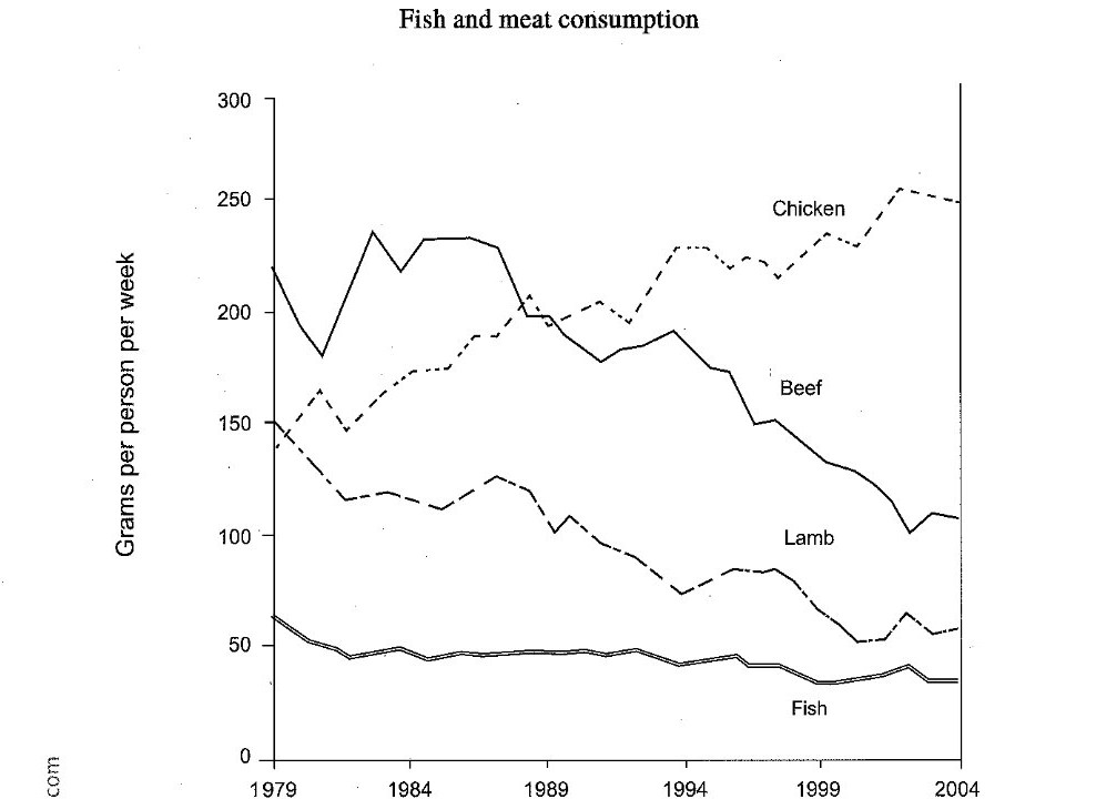
The line graph illustrates changes in the weekly consumption of fish, beef, lamb and chicken, measured in grams per person, from 1979 to 2004.
Overall, chicken consumption increased considerably and became the most popular meat by the end of the period. In contrast, beef and lamb consumption declined, while fish remained the least consumed food throughout the period.
In 1979, beef was the most widely consumed meat, at approximately 220 grams per person per week, while chicken and lamb stood at around 150 grams each. Beef consumption fluctuated during the early years, reaching a peak of about 230 grams in the early 1980s, before falling steadily to roughly 110 grams in 2004. Similarly, lamb consumption decreased from 150 grams to around 60 grams, despite some minor fluctuations over the period.
By contrast, chicken consumption showed an upward trend. Starting at approximately 140 grams per person per week, it fluctuated before rising significantly, overtaking beef around 1989. It then continued to increase, reaching about 250 grams by 2004. Meanwhile, fish consumption remained relatively stable compared with the other categories. It began at around 60 grams and gradually declined to approximately 35 grams at the end of the period, with only slight variations along the way.
Sample Question 7
Answer:
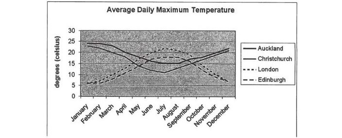
The line graph illustrates the average daily maximum temperatures, measured in degrees Celsius, in Auckland, Christchurch, London and Edinburgh over the course of a year, from January to December.
Overall, the temperatures in the two New Zealand cities followed a similar pattern, generally declining towards the middle of the year before rising again. In contrast, London and Edinburgh experienced warmer temperatures during the middle months, with London reaching the highest peak. The lowest temperatures were recorded at the beginning and end of the year in the European cities.
Auckland began the year at approximately 24°C, while Christchurch started at around 20°C. Both cities experienced a gradual decline in temperature, although Christchurch fell more sharply, reaching roughly 11°C in July and August. Auckland also decreased to about 15°C in June and July before recovering. Towards December, the temperatures in both cities rose, finishing at approximately 21°C in Auckland and 20°C in Christchurch.
London and Edinburgh started the year at around 5°C. Their temperatures increased steadily during the first half of the year, with London peaking at approximately 22°C in July and Edinburgh reaching about 20°C around the same period. Afterward, both cities experienced a decline. London fell to roughly 7°C in December, while Edinburgh ended the year at a similar level. Notably, London was generally warmer than Edinburgh during the summer months.
Sample Question 8
Answer:
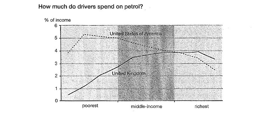
The line graph compares the percentage of income spent on petrol by drivers in the United States of America and the United Kingdom across three income groups: the poorest, middle-income and richest.
Overall, American drivers generally spent a higher proportion of their income on petrol than British drivers in the lower-income groups. However, the percentage for the UK increased with income, while the figure for the USA generally declined among richer drivers. The two figures became similar in the middle-income group.
Among the poorest drivers, Americans spent approximately 4% of their income on petrol, compared with only about 0.5% in the UK. The US figure rose to a peak of just over 5% before gradually falling to around 5%. Meanwhile, the proportion for British drivers increased steadily from 0.5% to approximately 3.5% as income rose.
In the middle-income group, UK drivers’ spending continued to rise, reaching nearly 4%, while the American figure declined to around 4%. Among the richest drivers, the UK percentage remained relatively stable at about 4% before dropping slightly to approximately 3.5%. In contrast, the US figure fell more sharply, declining from around 4% to just 3%. By the end, British drivers spent a slightly larger proportion of their income on petrol than their American counterparts.
Sample Question 9
Answer:
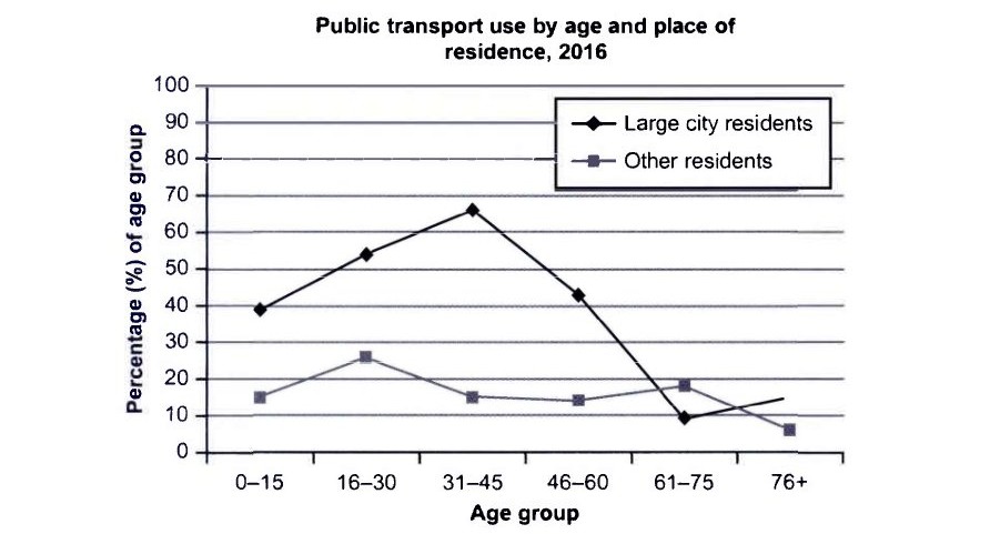
The line graph compares the percentages of people in six different age groups who used public transport in 2016, distinguishing between residents of large cities and those living in other areas.
Overall, public transport was considerably more popular among large-city residents, particularly those aged 31–45. By contrast, usage among other residents remained relatively low across most age groups. In both groups, the figures generally declined among older people.
Among large-city residents, approximately 39% of those aged 0–15 used public transport. This figure increased to around 54% for the 16–30 age group and reached a peak of about 66% among people aged 31–45. However, the percentage then fell sharply to roughly 43% for those aged 46–60. It dropped further to just 9% among people aged 61–75 before rising slightly to approximately 15% in the oldest group.
In comparison, public transport use among other residents stood at around 15% for the youngest age group and rose to a peak of approximately 26% among those aged 16–30. It subsequently declined to about 15% for people aged 31–45 and 14% for those aged 46–60. The figure then increased slightly to around 18% in the 61–75 age group before falling to approximately 6% among people aged 76 and above. Notably, other residents recorded higher usage than large-city residents in the 61–75 age group.
Sample Question 10
Answer:
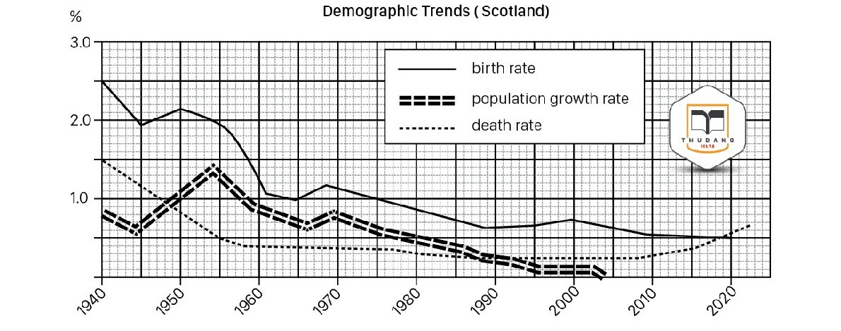
The line graph illustrates changes in the birth rate, death rate and population growth rate in Scotland between 1940 and 2023, measured in percentages.
Overall, all three rates declined considerably over the period. The birth rate remained the highest for most years, while the population growth rate fluctuated before falling to almost zero. In contrast, the death rate decreased initially but rose slightly towards the end.
In 1940, the birth rate stood at approximately 2.5%, compared with 1.5% for the death rate. The birth rate fell to around 2% in 1945 before briefly recovering. It then dropped sharply to about 1% in the early 1960s. After a slight increase around 1970, it continued declining, reaching roughly 0.5% by 2010.
The population growth rate peaked at approximately 1.4% in the mid-1950s before declining steadily to almost zero by the late 1990s. Meanwhile, the death rate fell to around 0.4% in the early 1960s and remained relatively stable for decades before increasing to approximately 0.6% by 2023.
Mistakes to Avoid
- Copying the question almost word for word in the introduction. Examiners notice this quickly, and it limits the vocabulary score.
- Leaving out the overview, or hiding it in the middle of the body. The reader should see the main trends straight away.
- Listing every data point. A string of numbers is not a report, and it leaves no room for comparison or selection.
- Offering opinions or guessing why the data changed. Task 1 asks you to describe what the graph shows, not to speculate about causes.
- Writing fewer than 150 words. Even accurate content can lose task achievement marks when the answer is too short to cover the key features properly.
Consistent practice is the key to improving your exam performance, and Gurully helps you make every practice session count. Strengthen your preparation with full-length mock tests and section-wise practice tests designed to help you build your skills. Get instant AI-powered scoring to identify your weak areas, understand your mistakes, and track where you need to improve. Experience real exam-like simulations, boost your confidence, and walk into your exam fully prepared.
FAQ:
How do I write an IELTS line graph answer?
How many words should an IELTS line graph answer be?
What is an overview in an IELTS line graph?
How is an IELTS line graph scored?
Is the line graph in IELTS General Training?
Also Read
Guide for IELTS Bar Graph – Tips, Template & Practice Questions
IELTS Writing Task 2 – Tips, Template & Sample Questions With Answers